Label errors are one of the most common yet overlooked sources of model brittleness. When training data contains systematic mislabeling, models learn to rely on spurious patterns rather than meaningful signals, leading to poor generalization and unexpected failures in production.

‍

Our SDK automatically detects these issues through representation-level analysis during training. By monitoring how model representations cluster around different examples and impact learning behavior, we can flag potential label errors without additional effort on your part. We run all of our analyses in the background and automatically surface causes of concern.

‍

‍

Getting Started

‍

Here’s how simple it is to start monitoring for label errors when training your model:

‍

Use the @tessel.arcana decorator to annotate your model class by specifying which layers to monitor. Then, our SDK will instrument your model to capture internal representations, predictions, and optional metadata such as labels and sample IDs. This process does not change your model’s forward logic and only needs to be implemented once for all of our analyses, even beyond label correction.

‍

import tessel, torch.nn as nn
from timm import create_model

@tessel.arcana(
    model_version=1.0,
    layer_mapping={
    	"features": "embedding", # representation from ViT backbone
    	"classifier_fc1": "fc1", # penultimate representation
    	"classifier_logits": "logits", # final logits
    },
 
    capture_labels=True,
    capture_sample_ids=True,
)
class TumorClassifier(nn.Module):
    def __init__(self, num_classes=2):
        super().__init__()
        backbone = create_model(
            "hf-hub:paige-ai/Virchow2", 
            pretrained=True
        ).eval().cuda()
        backbone.requires_grad_(False)
        
        self.embedding = lambda x: torch.cat(
            [x[:, 0], x[:, 5].mean(1)], 
            dim=-1
        ).float()
        self.backbone = backbone

‍

To activate logging, just wrap your inference or train loop with the tessel.context context manager and pass labels and sample_ids into the model’s forward call. You can log any intermediate layer by including it in the layer_mapping.

‍

sync_config = tessel.SyncConfig(
    sync_to_api=True,
    api_key="your_project_api_key",
    api_endpoint="https://api.tessel.ai/v1",
    run_name="virchow2_tumor_classification",
    auto_create_run=True,
)

with tessel.context(sync_config=sync_config):
    model = TumorClassifier(num_classes=2).cuda()
    model.eval()
    
    for images, labels, sample_ids in dataloader:
        images = images.cuda()
        outputs = model(
            images, 
            labels=labels, 
            sample_ids=sample_ids
        )

‍

Once you've added the decorator and wrapped your train or inference loop, you're done!

‍

There are no additional experiments to conduct or manual logs to configure. The SDK is integrated directly into your development workflow. Each time you train or evaluate, the SDK quietly collects the necessary data for downstream analysis and surfaces issues worth remediating. To log more data, you can simply update the config to include additional layers and metadata.

‍

With the data logged, you can run label error detection with a single call:

‍

import tessel

# Run-level label error detection (within-run or cross-run)
errors, metadata = tessel.detect_label_errors(
    run_id="virchow2_tumor_classification"
)
print(errors[:1])

‍

This returns a list of suspicious samples (errors), along with a metadata object that describes the analysis setup. The metadata includes which runs were analyzed, how many classifiers were trained, how many cross-validation folds were used, how neighborhoods were defined, how final scores were aggregated, and other method-specific configuration details. We also provide a dashboard-level view through our web platform to visually understand exactly what’s happening.

‍

‍

Case Study in Digital Pathology

‍

Background

‍

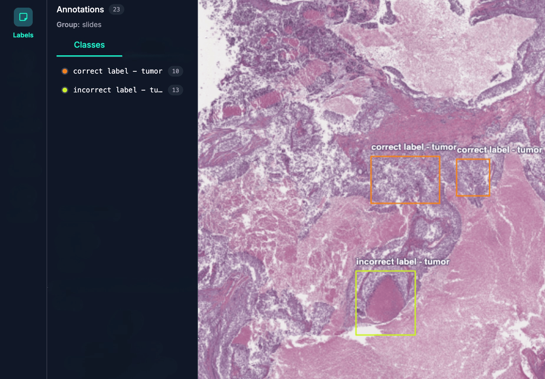
To see the SDK in action, we run a case study to demonstrate label error detection on a breast cancer metastases classification task in digital pathology. This is a domain where label errors are particularly common and can significantly impact model reliability. For example, a slide labeled as “tumor” could be incorrect due to any number of reasons:

‍

• Genuine human error
• Disagreement among pathologists on classification
• Differences in labeling methodology
  
  • One dataset provider might label tumor-adjacent patches as “tumor” even without clear tumorous signal
  • Another dataset might label similar patches as “normal”

‍

These inconsistencies make it difficult for the model to learn robust class boundaries. Consequently, when the model encounters new data, such as slides from a hospital outside the model’s train distribution, its behavior can be erratic and fail to generalize.

‍

Representation analysis helps identify these issues early on. Mislabeled or ambiguous examples leave distinct traces in representation space. These examples may appear isolated from their class cluster, be grouped with the wrong class, or show unusually high loss when a lightweight label classifier is trained on the representations. Our tools automatically identify these outliers, allowing you to review potential labeling errors without manually inspecting thousands of examples or wasting expert time on annotating flawed data.

‍

‍

Setup

‍

Model: We use Virchow2, a state-of-the-art pathology foundation model, as our backbone and attach a linear head for binary tumor/normal prediction. The classifier is trained on mean patch embeddings, obtained by averaging Virchow2 embeddings across all patches from a slide.

‍

Dataset: We use a patch-based variant of Camelyon17 from the WILDS benchmark, a dataset of 96×96-pixel histopathological patches from lymph node sections labeled "tumor" or "normal." The dataset includes metadata on the patch's hospital of origin, which accounts for systematic differences due to staining protocols and hardware. Following the benchmark design, we split the data by hospital: three centers for training, one for validation, and one for testing. We opted to use 10% of the dataset for both train and validation to emulate a low data regime while still evaluating on the full test set. This reduced-data setting still retains sufficient learning signal, as a linear classifier on mean patch embeddings achieves 98% accuracy on the test set. 

‍

Limitations: The original Camelyon17 dataset does not contain confirmed mislabelings, which are a common challenge in real-world medical data. To address this, we introduce synthetic label flips to create controlled error conditions for our experiments.

‍

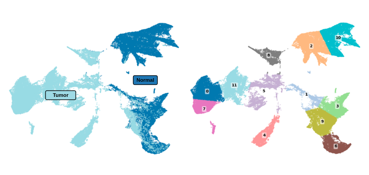
Simulating Systematic Errors: To simulate realistic mislabeling, we reduce the train set Virchow2 embeddings to two dimensions using UMAP and then cluster them into 12 groups with k-means. This process reveals that the model clearly separates tumor and normal tissue in its representation space. We then strategically flipped the labels of 20% of the "tumor" samples from a single cluster to "normal."

‍

‍

While this is a synthetic simulation, it serves as a meaningful proxy for real-world mislabeling, which often arises from non-random factors like disagreements among pathologists or inconsistent labeling protocols. These factors introduce systematic biases that disproportionately affect specific subsets of the data. We focus on tumor-to-normal flips because a missed tumor (false negative) carries far more serious consequences than a false positive in clinical settings.

‍

We are currently curating a high-quality dataset that captures real-world pathology mislabeling and will re-test this approach. If you have such a dataset and are interested in collaborating, please reach out to us at team@tessel.ai.

‍

We repeat this experiment across all clusters in the training data that contain tumor examples and evaluate both our ability to detect these errors and their impact on classifier performance. 

‍

Comparison and Analysis: To properly analyze the impact of label error detection, we compare three versions of the model:

‍

1. Baseline Model: We train a classifier on the data with 20% of "tumor" samples in a single cluster synthetically flipped to "normal." This represents the performance of a model trained on noisy data.
2. Corrected Model: We apply our SDK to detect and flag these label errors. After flipping the flagged points to their correct class, we retrain the classifier head on the corrected data. This demonstrates the impact of our error detection and correction process.
3. Upper Bound Model: We also train a classifier on the original, clean dataset to establish an upper performance bound. It is important to note that when using our SDK in production, this step is not present. We simply use it in the case study as a reference for viewers.

‍

It’s important to note that when comparing these models, it is grossly inadequate to just look at dataset-level metrics. To illustrate this, we conduct representation analysis by applying the same UMAP and k-means clustering procedure that we applied to the train set to the test set.

‍

‍

This enables us to look beyond high level performance and actually investigate cluster-specific effects. This is a critical step because systematic mislabelings will produce disproportionate effects on specific subgroups (e.g. samples scanned by a specific brand of scanner), even if overall accuracy is still high. By analyzing performance at the cluster level within the representation space, we can expose and quantify these hidden failure modes.

‍

‍

Results & Insights

‍

We explicitly choose not to report the percentage of label errors detected because it’s not what we actually care about. Our goal is a more robust model on the downstream task of choice, not necessarily a perfect dataset. These two are likely correlated but distinct nonetheless.

‍

This is central to our belief in rethinking model evaluation from a clinical perspective rather than an academic one. As such, our metric of focus is the recovery of downstream performance following the correction of detected mislabeled clusters. This provides a better look at tangible changes in model behavior and helps us quantify the clinical impact of more detected label errors rather than another uninterpretable number.

‍

As expected, we find that the injected label errors do not significantly affect overall classifier performance. Across all corruption experiments, test accuracy only dropped modestly—from 98.4% in the clean setting to between 95.5% and 98.0%. This is because corrupting 20% of a single cluster only touches about 3% of the entire dataset, so the dominant tumor-normal signal remains intact and the model maintains high accuracy.

‍

However, this obscures the real problems. A model can have near-perfect overall performance while still failing catastrophically on specific subgroups. To expose these issues, we evaluate performance at the cluster level by aligning corrupted training regions with semantically meaningful test clusters.

‍

Main failure mode:

‍

• Train cluster 9 corruption (worst case):
  
  • Test cluster 4 collapses from 99.8% → 64.6% (–35.2%). With our label detection algorithm, it recovers to 99.7%, i.e. >99% of the impact mitigated

‍

‍

Additional performance drops we found:

‍

• Train cluster 0 corruption:
  
  • Test cluster 4 dropped from 99.8% → 83.6% (–16.2%), recovered to 99.6%, i.e. 99% of the loss corrected
  • Test cluster 8 dropped from 94.3% → 85.3% (–9.0%), recovered to 94.3%, i.e. 100% of the loss corrected
    
    
• Train cluster 5 corruption:
  
  • Test cluster 4 dropped from 99.8% → 82.3% (–17.5%), recovered to 99.8%, i.e. 100% of the loss corrected
    
    
• Train cluster 8 corruption:‍
  
  • Test cluster 4 dropped from 99.8% → 88.2% (–11.6%), recovered to 99.7%, i.e. 99% of the loss corrected
  • Test cluster 8 dropped from 94.3% → 93.6% (–0.7%), recovered to 93.8%, i.e. almost full recovery

‍

In real-world examples, we can imagine that these clusters correspond to biological or slide preparation differences. Systematic mislabeling would then cause critical failures within that subgroup that are not reflected in dataset-level metrics, ultimately causing adverse clinical outcomes. This is the kind of failure mode that model providers should be responsible for reporting and fixing rather than glossing over with blanket metrics. When analyzing real-world label errors, it is important to baseline findings with pathologist insight. But even just leveraging available metadata and carefully describing model behavior in context, we can generate insights that flag odd behavior for further review and directly guide optimization.

‍

As shown, our SDK can achieve recovery without access to the ground truth; it simply reverses the examples flagged during the analysis. Even when some correct samples are mistakenly flagged, the downstream classifier remains unaffected because the dominant tumor-normal signal and the decision boundary both remain intact. Similarly, recovery succeeds even when not all corrupted samples are detected because enough harmful labels are corrected to neutralize the corrupted cluster’s influence. In practice, perfect detection is not required; as long as the majority of errors in the affected region are flagged, the procedure consistently restores performance, often matching or approaching the clean upper bound. This demonstrates that targeted correction at the representation level is sufficient to recover downstream accuracy, even with imperfect detection. We believe this is the perfect example of choosing the right metric to serve as a proxy for clinical outcome.

‍

‍

What’s Next

‍

Neural representation analysis extends far beyond label error detection. The same representations we extract for identifying mislabeled samples can power distribution shift detection at inference time, automated quality control flagging, and model lifecycle monitoring. Behind the scenes, we’re building an ecosystem where the neural representations you’re already logging unlock an expanded suite of analytical and actioning capabilities.

‍

A compelling example came from a histologist we collaborated with during this research. He noted that “any sample that is not a textbook example in H&E staining is flagged for further IHC staining to identify more specific cancer markers”. This perfectly captures the potential: at scan time, patches can already be screened using representation analysis to automatically detect samples requiring additional scrutiny. This encompasses processing artifacts (tears, folds, wax-processing issues), non-standard biology, or cases that fall outside typical diagnostic patterns.

‍

Beyond expanding use cases, we’re also advancing the analytical methods themselves. The representation analysis we performed in this case study was quite straightforward–UMAP and k-means clustering. This is nothing novel, it’s a routine procedure that data science teams already commonly employ for analysis. We have developed novel approaches built on the latest mechanistic interpretability research that enables us to decompose complex high dimensional spaces into specific subsets of dimensions that correlate to both biological and spurious signals. This opens unprecedented possibilities for model explanation and iterative improvement. 

‍

The promise of our SDK for neural representation logging and analysis is a future where evaluation becomes continuous and adaptive rather than static. The constant accumulation of model insights becomes your de-facto source for understanding behavior, replacing reliance on fixed benchmarks with dynamic assessments rooted in desired outcomes. As machine learning techniques advance and interpretability methods improve, every SDK user automatically benefits from these innovations without additional engineering overhead. This creates a powerful feedback loop: better models generate richer representations, richer representations enable more sophisticated evaluations, and the right evaluations provide clear signals for optimization. The ultimate goal is models that are not only robust, but truly understand their own capabilities and limitations. This is trustworthy evaluation infrastructure built for the long term, designed to scale with your organization and get smarter over time.

‍